# The cheapest plan wins
> Follow a query from SQL to plan, check the planner's arithmetic by hand, and see exactly why it picks each scan, join, worker count, and JIT.
---
LLMS index: [llms.txt](/en/llms.txt)
---
Here is a join every multi-tenant app writes sooner or later. Every row carries `account_id`, so you match on it everywhere, just to be safe:
```sql
select count(*)
from events e
join projects p on p.id = e.project_id and p.account_id = e.account_id
join users u on u.id = p.owner_id and u.account_id = p.account_id;
```
The tenant conditions are redundant: a project belongs to one account, and so does its owner. They change nothing about the answer. They change the plan completely:
```text
Aggregate (cost=67569.72..67569.73 rows=1 width=8)
(actual time=3366.344..3366.347 rows=1.00 loops=1)
Buffers: shared hit=5998602 read=36762
-> Nested Loop (cost=691.29..67569.72 rows=2 width=0)
(actual time=3.700..3268.819 rows=2000000.00 loops=1)
```
The planner expected 2 rows and got 2,000,000. It picked a plan that's perfect for 2 rows and touched 6,035,364 pages. Drop the redundant conditions and the same count reads 36,490.
[The planner is guessing](/en/20-planner/#basics-chapter-20) covered the estimates. This chapter is what the planner does with them, and the news is reassuring: it isn't clever, it's consistent. It picks the cheapest plan it can price, and every choice is arithmetic you can check. When the plan is bad, a price or a row count was wrong, and you can find which.
Plans are from PostgreSQL 18, with parallelism and JIT off unless the section is about them.
## Your query is rewritten before it's priced
Before a single cost is computed, your query has already been rewritten twice:
```text
SQL
|
v
parse resolve names and types against the catalog
|
v
rewrite views become subqueries; RLS policies become
| WHERE conditions
v
preprocess (no costs yet, only logic)
| - pull subqueries and IN/EXISTS up into joins
| - push filters down toward the tables
| - fold constants, drop contradictions
| - turn outer joins into inner joins
| - remove joins nobody reads; inline CTEs
| - PG 18: remove self-joins, OR lists to ANY
v
paths every way to scan each table, every join
| order and method, priced; cheapest survives
v
plan one tree, plus the JIT decision
```
Every rewrite gives the search a simpler problem, and every one shows in `EXPLAIN`. So **don't hand-optimize what the preprocessor already does.** `IN (subquery)` becomes a join the planner can reorder, and a CTE used once is inlined ([CTEs: inlined or materialized](/en/22-queries/#a-cte-used-once-is-inlined-not-fenced)).
### Views and policies are text substitution
A view is a stored query pasted into yours, so it costs nothing at run time. A [row-level security](/en/43-glossary/#row-level-security) policy is pasted in the same way, as one more `WHERE` condition: the policy you never wrote shows up as the `Index Cond`, which is why the tenant column needs an index ([RLS performance: policies are predicates](/en/33-security/#rls-performance-policies-are-predicates)). One exception to "costs nothing": policies and `security_barrier` views won't let your own conditions run before theirs unless the functions in them are marked `leakproof`, so a filter that would have been pushed down into an index can end up checked row by row.
### Constants are folded
Expressions with no column in them are computed once, at plan time: `where id = 2 * 21` becomes `Index Cond: (id = 42)`, and `and 1 = 2` plans to a `Result` with `One-Time Filter: false` that reads nothing. Stable functions like `now()` aren't folded (a prepared statement might run tomorrow), but the planner evaluates them to estimate rows, which is why `created_at >= now() - interval '1 day'` gets a real estimate and an index.
> [!DETAILS]- Deep dive: Each rewrite, seen in EXPLAIN
>
> **Filters move down.** A filter on a grouped subquery's grouping column lands below the aggregate, so Postgres counts one project's rows, not all 20,000 projects' rows before throwing 19,999 away (`GroupAggregate` over `Seq Scan ... Filter: (project_id = 42)`).
>
> **Outer joins become inner joins.** `projects p left join events e ... where e.kind = 'deploy'` can't keep the empty projects (their `e.kind` is null), so it's planned as a plain `Hash Join` the search can reorder. If you meant to keep them, the filter belongs in the `ON` clause.
>
> **Joins nobody reads disappear.** `select p.* from projects p left join users u on u.id = p.owner_id` plans to `Seq Scan on projects p` alone. ORMs generate joins like this constantly, and this rewrite is why those joins cost less than they look.
>
> **PostgreSQL 18 removes self-joins and folds `OR` lists.** A table joined to itself on its primary key loses the second scan, and `id = 1 or id = 2 or id = 3` becomes one probe, `Index Cond: (id = ANY ('{1,2,3}'::integer[]))`.
>
> > [!EXAMPLE]- Prove it · lab `20-plans`
> >
> > ```sql
> > select lab.prove('a filter on a grouped subquery is pushed below the aggregate',
> > lab.est_nodes($$ select * from (select project_id, count(*) from events
> > group by project_id) s
> > where project_id = 42 $$) = '{Aggregate,Seq Scan}'
> > and lab.est_rows($$ select * from (select project_id, count(*) from events
> > group by project_id) s
> > where project_id = 42 $$) = 1);
> >
> > select lab.prove('an unused LEFT JOIN to a unique key is removed entirely',
> > lab.est_nodes($$ select p.* from projects p left join users u on u.id = p.owner_id $$)
> > = '{Seq Scan}');
> >
> > select lab.prove('PostgreSQL 18 removes a self-join on the primary key',
> > lab.est_nodes($$ select e1.* from events e1 join events e2 on e2.id = e1.id
> > where e2.kind = 'deploy' and e1.id < 100 $$) = '{Index Scan}');
> > ```
> >
> > [Full lab script](https://www.flagon.io/books/eight-kilobytes/lab/20-plans.sql)
## Errors compound up the join tree
Back to the opening query. A join's estimate is its inputs multiplied by a [selectivity](/en/43-glossary/#selectivity), and with two join conditions the planner multiplies both as if they were independent ([The planner assumes your columns are independent](/en/20-planner/#the-planner-assumes-your-columns-are-independent)):
```text
events x projects 2,000,034 x 20,000
x 1/20,000 (e.project_id = p.id)
x 1/1,000 (e.account_id = p.account_id)
= about 2,000 rows (actual: 2,000,000)
```
The second condition removes nothing, so the estimate is 1,000 times too low. Then the error becomes an *input*. The join to `users` has its own redundant condition and divides by about 1,000 again: 2 rows. For 2 rows, a nested loop probing `users` by index is the right plan. For 2,000,000 it's two million probes, about three pages each.
Without the redundant conditions, every estimate is right, both joins hash, and the query reads 165 times fewer pages. A 10x error at two levels is 100x by the third.
> [!WARNING] Redundant join conditions are not free
>
> Matching on `account_id` in every join feels safe, and ORMs with composite keys generate it. Each redundant condition divides the estimate by its column's distinct count. Join on the key that determines the row. To guarantee the account matches, use a composite foreign key, `events (project_id, account_id) references projects (id, account_id)`: it constrains the data, and the planner reads foreign keys when it estimates joins, so with it in place the two-condition join is estimated correctly too.
> [!DETAILS]- Deep dive: The two plans, side by side
>
> ```text
> -> Nested Loop (... rows=2 ...) (actual ... rows=2000000.00 loops=1)
> -> Hash Join (... rows=1999 ...) (actual ... rows=2000000.00 loops=1)
> Hash Cond: ((e.project_id = p.id) AND (e.account_id = p.account_id))
> -> Index Scan using users_pkey on users u (... rows=1 ...)
> (actual ... rows=1.00 loops=2000000)
> ```
>
> Without the redundant conditions:
>
> ```text
> Buffers: shared hit=1126 read=35364
> -> Hash Join (... rows=2000034 ...) (actual rows=2000000.00 loops=1)
> ```
>
> The `users` hash cost the 1,126 hits (the whole `users` table), and the reads are `events` plus `projects`. The check below also confirms the composite foreign key fix from the callout.
>
> > [!EXAMPLE]- Prove it · lab `20-plans`
> >
> > ```sql
> > select lab.prove('a redundant tenant clause divides the join estimate by about 1,000',
> > lab.est_rows($$ select * from events e join projects p
> > on p.id = e.project_id and p.account_id = e.account_id $$)
> > between 1500 and 2500
> > and lab.est_rows($$ select * from events e join projects p on p.id = e.project_id $$)
> > > 1900000);
> >
> > select lab.prove('the compounded misestimate costs over 100x the pages of the plain join',
> > lab.buffers($$ select count(*) from events e
> > join projects p on p.id = e.project_id and p.account_id = e.account_id
> > join users u on u.id = p.owner_id and u.account_id = p.account_id $$)
> > > 100 * lab.buffers($$ select count(*) from events e
> > join projects p on p.id = e.project_id
> > join users u on u.id = p.owner_id $$));
> >
> > begin;
> > alter table projects add constraint projects_id_account_key unique (id, account_id);
> > alter table events add constraint events_project_account_fkey
> > foreign key (project_id, account_id) references projects (id, account_id);
> > analyze projects;
> > select lab.prove('with a composite foreign key, the two-condition join is estimated at about 2 million rows',
> > lab.est_rows($$ select * from events e join projects p
> > on p.id = e.project_id and p.account_id = e.account_id $$) > 1900000);
> > rollback;
> > ```
> >
> > [Full lab script](https://www.flagon.io/books/eight-kilobytes/lab/20-plans.sql)
## Access paths are priced, not ranked
For each table, the planner builds every scan it could use ([three ways to read an index](/en/17-btree/#an-index-helps-only-as-much-as-its-rows-sit-together), plus the sequential scan) and prices each one. There's no rule that says "index beats sequential". There's arithmetic, and the number that moves it most is [correlation](/en/43-glossary/#correlation).
### Correlation prices the index scan
An index scan's I/O cost slides between two extremes. At correlation 0, every matching row sits on a different page, fetched in random order. At correlation 1, matching rows sit on consecutive pages, read nearly in order. The planner slides by **correlation squared**, so only a strong correlation earns much of the discount: at 0.5 you get a quarter of it.
To isolate it, give `events` an index on `created_at` and copy the table in random order with the same index: same rows, only the physical order differs. Forced into an index scan for the last day of events (bitmap scans switched off for the session), the shuffled copy costs 82 times as much, and left alone the planner picks a bitmap scan instead.
### The 5% rule is wrong in both directions
Widen the window and each table switches plans at some width:
| Table | Plan | Until (window) | Estimated rows |
|---|---|---|---|
| events (correlation 1) | Index Scan | 235 days | 1,293,301 (65%) |
| events (correlation 1) | Seq Scan | beyond | |
| events_shuffled | Index Scan | 2 minutes | 8 |
| events_shuffled | Bitmap Heap Scan | 143 days | 781,520 (39%) |
| events_shuffled | Seq Scan | beyond | |
**Table 21-1.** The 5% rule is wrong in both directions
So much for "use an index for under 5% of the table." On ordered data the index scan held out to 65% of the table. On shuffled data a plain index scan won only for a handful of rows, and the bitmap scan held on to 39%, because once it touches most pages it reads them in physical order.
At the flip points on our machine, with everything cached, the sequential scan was actually faster than the plan it replaced (about 115 ms against 210 ms at the ordered table's flip): the argument for a lower `random_page_cost` when your data fits in memory, set once for the whole server.
> [!DETAILS]- Deep dive: The interpolation, and the experiment behind the table
>
> ```text
> max_IO = pages fetched x random_page_cost (correlation 0)
> min_IO = 1 x random_page_cost
> + (rest of the pages) x seq_page_cost (correlation 1)
>
> IO cost = max_IO - correlation^2 x (max_IO - min_IO)
> ```
>
> ```sql
> create index events_created_at_idx on events (created_at);
> create table events_shuffled as select * from events order by random();
> create index events_shuffled_created_at_idx on events_shuffled (created_at);
> analyze events_shuffled;
> -- correlation of created_at: 1 on events, -0.004 on events_shuffled
> ```
>
> For `created_at >= '2026-10-05'`, forcing an index scan on both:
>
> ```text
> Index Scan using events_created_at_idx on events
> (cost=0.43..242.75 rows=5104 width=112)
>
> Index Scan using events_shuffled_created_at_idx on events_shuffled
> (cost=0.43..19884.52 rows=5304 width=112)
> ```
>
> Left alone, the shuffled table gets a bitmap scan at 14,360. The lab finds each flip in the table by binary search over the window width. Index-only scans get their own discount for all-visible pages, priced from `pg_class.relallvisible`.
>
> > [!EXAMPLE]- Prove it · lab `20-plans`
> >
> > ```sql
> > select lab.prove('correlated: the index scan holds until 50 to 80 percent of the table, then a seq scan',
> > path_at('events', 60) = 'Index Scan'
> > and path_at('events', current_setting('plans.flip_corr')::int + 1) = 'Seq Scan'
> > and rows_at('events', current_setting('plans.flip_corr')::int)
> > / (select reltuples from pg_class where relname = 'events') between 0.5 and 0.8);
> >
> > select lab.prove('shuffled: index scan only for a handful of rows (under 100), then bitmap',
> > path_at('events_shuffled', 1) = 'Index Scan'
> > and path_at('events_shuffled', current_setting('plans.flip_ib')::int + 1) = 'Bitmap Heap Scan'
> > and rows_at('events_shuffled', current_setting('plans.flip_ib')::int) < 100);
> >
> > select lab.prove('shuffled: bitmap until 20 to 60 percent of the table, then a seq scan',
> > path_at('events_shuffled', current_setting('plans.flip_bs')::int + 1) = 'Seq Scan'
> > and rows_at('events_shuffled', current_setting('plans.flip_bs')::int)
> > / (select reltuples from pg_class where relname = 'events_shuffled') between 0.2 and 0.6);
> > ```
> >
> > [Full lab script](https://www.flagon.io/books/eight-kilobytes/lab/20-plans.sql)
## Sorted order is a property of a path
A path also carries the order its rows come out in (the planner calls it **pathkeys**), so a costlier path survives the search if its order might save a sort later. `ORDER BY ... LIMIT` is where that pays. `order by created_at desc limit 10` walks the index backward and stops after 4 pages; the `Limit` pays only for the fraction it reads. Ask for an order no index provides (`order by kind, created_at desc`) and every row is read and sorted before the first comes out: 35,179 pages.
In between, an **incremental sort** (PostgreSQL 13+) uses an index for the first sort key and sorts within each group: `order by created_at desc, kind limit 10` read 8 pages.
An unexpected sort means no path produced the order ([Limit bets on finding rows early](/en/19-explain/#limit-bets-on-finding-rows-early) shows the expensive version).
> [!DETAILS]- Deep dive: Three ORDER BY ... LIMIT plans
>
> The backward index scan reported `Buffers: shared read=4` and the sort `shared hit=6 read=35173`; the incremental sort showed `Presorted Key: created_at`. The first index scan's total cost is 87,124, but its `Limit` costs 0.86. The sort's startup cost (98,392) is nearly its total: nothing comes out until it has seen every row.
>
> > [!EXAMPLE]- Prove it · lab `20-plans`
> >
> > ```sql
> > select lab.prove('ORDER BY created_at DESC LIMIT 10 walks the index backward: no Sort, under 20 pages',
> > lab.est_nodes($$ select id, kind, created_at from events
> > order by created_at desc limit 10 $$) = '{Limit,Index Scan}'
> > and lab.buffers($$ select id, kind, created_at from events
> > order by created_at desc limit 10 $$) < 20);
> >
> > select lab.prove('ORDER BY created_at DESC, kind LIMIT 10 uses an incremental sort on the index order',
> > lab.est_nodes($$ select id, kind, created_at from events
> > order by created_at desc, kind limit 10 $$)
> > = '{Limit,Incremental Sort,Index Scan}'
> > and lab.buffers($$ select id, kind, created_at from events
> > order by created_at desc, kind limit 10 $$) < 20);
> > ```
> >
> > [Full lab script](https://www.flagon.io/books/eight-kilobytes/lab/20-plans.sql)
## Join order is a search, and searches get expensive
With the cheapest paths for each table in hand, the planner looks for the cheapest way to combine them, the way the 1979 System R paper laid out: dynamic programming. Find the best plan for every pair of tables, extend each by one table, and keep only the cheapest plan per set of tables. That pruning makes the search feasible. It still grows fast. Here are 4 to 13 copies of a 1,000-row table, all joined on one key, planned exhaustively (`geqo = off`) and with default settings:
| Tables | Planning, exhaustive | Planning, default settings |
|---|---|---|
| 4 | 0.4 ms | 0.5 ms |
| 8 | 8.1 ms | 10.5 ms |
| 10 | 75.7 ms | 112.5 ms |
| 11 | 217 ms | 211 ms |
| 12 | 962 ms | 41.8 ms |
| 13 | 2,609 ms | 37.6 ms |
**Table 21-2.** Join order is a search, and searches get expensive
Each extra table roughly triples exhaustive planning, until 12 tables, where the default column falls off a cliff. That's `geqo_threshold = 12`: from there the **genetic query optimizer** (GEQO) replaces exhaustive search with a randomized one that stops after a fixed effort. Planning stays flat; the plan is good rather than guaranteed best.
`join_collapse_limit` (default 8) keeps big queries from the full search: explicit `JOIN`s beyond 8 items are planned in chunks, each optimal, in your written order. The same 12 tables as explicit `JOIN ... ON` planned in 9.2 ms against 962 ms for the comma list planned exhaustively. So the exhaustive search reaches 11 tables only for comma lists; with `JOIN` syntax, which is what ORMs write, it stops at 8. `join_collapse_limit = 1` makes the planner follow your join order exactly. Touch these per session, never globally. And past a dozen tables, check `Planning Time` before you blame the executor: an ORM's eager load can spend more time planning than running.
> [!DETAILS]- Deep dive: Measuring planning time
>
> Best of three runs on our machine; the shape matters, not the digits. GEQO seeds from `geqo_seed`, so the same query and statistics get the same plan.
>
> > [!EXAMPLE]- Prove it · lab `20-plans`
> >
> > ```sql
> > select lab.prove('exhaustive planning time grows steeply: 11 tables take over 10x as long as 7',
> > current_setting('plans.ms11')::numeric > 10 * current_setting('plans.ms7')::numeric);
> >
> > select lab.prove('at 12 tables GEQO takes over, planning at least 3x faster than exhaustive search',
> > current_setting('plans.ms12')::numeric > 3 * current_setting('plans.ms12g')::numeric);
> >
> > select lab.prove('explicit JOINs past join_collapse_limit (8) are planned in pieces, far faster',
> > current_setting('plans.ms12')::numeric > 5 * current_setting('plans.ms12j')::numeric);
> > ```
> >
> > [Full lab script](https://www.flagon.io/books/eight-kilobytes/lab/20-plans.sql)
## Each join method wins on a cost curve
[Each join method is right only for some row counts](/en/19-explain/#each-join-method-is-right-only-for-some-row-counts) shows how to read the three join nodes. Here's why each gets picked:
```text
nested loop cost ~ outer rows x (cost of one inner lookup)
grows linearly with the outer side
hash join cost ~ build inner hash + scan outer once
mostly fixed; jumps if it needs batches
merge join cost ~ sort both sides (unless already sorted)
+ one pass over each
```
The planner prices all three for every pair and keeps the cheapest, so the choice moves when row counts move. One account's 20 projects joined to their events is a nested loop: each project costs an index lookup of about 383 units, where a hash join would scan all of `events` (about 55,000) first. Widen it to `account_id <= k`: at 8 accounts (190 projects) it's still a nested loop; at 9 (212) it flips to a hash join.
That's also why a nested loop is the most dangerous plan when the outer estimate is low: it's chosen for small numbers, and its cost grows with the real count.
Memory moves the choice too, and not always where you'd look. Joining all of events to users `order by e.user_id` is a merge join at the default [`work_mem`](/en/43-glossary/#work_mem) of 4 MB. The hash join isn't the problem: the 100,000-user hash fits in one batch at 4 MB, because `hash_mem_multiplier` gives a hash twice `work_mem`, and the hash join is priced the same at 4 MB and 8 MB. The problem is the sort the hash join needs afterward: two million joined rows, about 35 bytes each, sorted on disk. The merge join sorts only the narrow `events` side (14 bytes a row) before joining, so at 4 MB it's cheaper. At 8 MB the big sort needs fewer merge passes, its estimate drops, and the same query becomes a hash join plus a sort: one setting, a different join, which is a good reason to raise `work_mem` for a reporting role rather than the whole server.
**Memoize** (PostgreSQL 14+) is a nested loop with a memory: a cache over the inner side, keyed by the join value, added when the outer side's distinct keys are far fewer than its rows. In its plan node, `Misses` are real executions of the inner side and `Hits` are executions saved. Archived projects, each with its account's user count: 3,911 outer rows but 989 distinct accounts, so the subquery ran 989 times, and the query read 3,444 pages instead of 13,075 with `enable_memoize = off`. Its input to watch is `n_distinct` on the join column.
> [!DETAILS]- Deep dive: The crossover, the merge join, and the Memoize
>
> The single-account nested loop's inner side is a **parameterized path**: an index scan (`Index Cond: (project_id = p.id)`) that takes its key from the current outer row, which is why nested loops are fast. At `k = 8` the nested loop costs 60,105; at `k = 9` the hash join costs 60,688. The crossover is around 19,000 events, 1% of the table. At 4 MB the merge join costs 371,832, against 387,490 for the hash join plus sort; at 8 MB the hash join plus sort costs 332,802. Inside both, the hash join itself costs 63,799 and ran in one batch using 7,274 KB, the same hash the previous chapter ran in one batch ([Each join method is right only for some row counts](/en/19-explain/#each-join-method-is-right-only-for-some-row-counts)). The whole difference is the sort on top: 382,490 to start at 4 MB, 327,802 at 8 MB, for a sort that spilled about 96 MB either way. The Memoize node:
>
> ```text
> -> Memoize (cost=6.43..6.44 rows=1 width=8) (actual rows=1.00 loops=3911)
> Cache Key: p.account_id
> Hits: 2922 Misses: 989 Evictions: 0 Overflows: 0 ...
> ```
>
> > [!EXAMPLE]- Prove it · lab `20-plans`
> >
> > ```sql
> > select lab.prove('more outer rows flip it to a hash join, somewhere between 2 and 30 accounts',
> > current_setting('plans.nl_flip')::int between 2 and 30
> > and join_node($$ select count(e.payload) from projects p
> > join events e on e.project_id = p.id where p.account_id <= 50 $$) = 'Hash Join');
> >
> > set work_mem = '4MB';
> > select lab.prove('at work_mem 4MB, events x users ORDER BY user_id is a merge join',
> > join_node($$ select e.kind, u.email from events e join users u on u.id = e.user_id
> > order by e.user_id $$) = 'Merge Join');
> > select set_config('plans.merge_cost', est_cost($$ select e.kind, u.email from events e
> > join users u on u.id = e.user_id order by e.user_id $$)::text, false) \g /dev/null
> > set enable_mergejoin = off;
> > select set_config('plans.hj4', hj_cost($$ select e.kind, u.email from events e
> > join users u on u.id = e.user_id order by e.user_id $$)::text, false),
> > set_config('plans.hashsort4', est_cost($$ select e.kind, u.email from events e
> > join users u on u.id = e.user_id order by e.user_id $$)::text, false) \g /dev/null
> > select lab.prove('at 4MB the rejected hash join plus sort costs more than the merge join',
> > join_node($$ select e.kind, u.email from events e join users u on u.id = e.user_id
> > order by e.user_id $$) = 'Hash Join'
> > and current_setting('plans.hashsort4')::numeric
> > > current_setting('plans.merge_cost')::numeric);
> > reset enable_mergejoin;
> > set work_mem = '8MB';
> > select lab.prove('at work_mem 8MB the same query becomes a hash join plus a sort',
> > join_node($$ select e.kind, u.email from events e join users u on u.id = e.user_id
> > order by e.user_id $$) = 'Hash Join');
> > select lab.prove('the hash join costs the same at 4MB and 8MB; only the sort above it got cheaper',
> > hj_cost($$ select e.kind, u.email from events e join users u on u.id = e.user_id
> > order by e.user_id $$) = current_setting('plans.hj4')::numeric
> > and est_cost($$ select e.kind, u.email from events e join users u on u.id = e.user_id
> > order by e.user_id $$) < current_setting('plans.hashsort4')::numeric);
> > ```
> >
> > [Full lab script](https://www.flagon.io/books/eight-kilobytes/lab/20-plans.sql)
## Parallel plans are priced like everything else
A parallel plan is one more path with two extra prices: `parallel_setup_cost` (1000) to start the workers and `parallel_tuple_cost` (0.1, ten times `cpu_tuple_cost`) for each row a worker hands the leader. So small tables never qualify, scans returning millions of rows rarely do, and scans that boil down to a few rows are the sweet spot.
The worker count comes from the table's size, not the query: one worker at 8 MB (`min_parallel_table_scan_size`), one more each time the table triples, so `events` at 275 MB rates 4, capped by `max_parallel_workers_per_gather` (default 2).
### One unlabeled function keeps a query serial
The planner refuses a parallel plan for queries that write or lock rows (`create table ... as` and `create materialized view` are the exceptions: their `select` can go parallel), for cursors, and for any query calling a function marked `PARALLEL UNSAFE`, and **user-defined functions are `PARALLEL UNSAFE` by default**. One unlabeled helper in a `WHERE` clause, and a two-million-row scan runs in one process. Mark pure computations `parallel safe` ([Parallel safety is opt-in](/en/24-functions/#parallel-safety-is-opt-in)).
> [!DETAILS]- Deep dive: Workers by table size, and the unsafe function, measured
>
> The same `count(*)` on copies of `events`, with `max_parallel_workers_per_gather = 8` and both parallel costs at zero so the planner always goes parallel: `projects` (1.5 MB) got none; copies of 10, 28, and 83 MB got 1, 2, and 3 workers; `events` (275 MB) got 4. With default costs, `ev_70k` gets no parallel plan at all. Override the size rule per table with `alter table events set (parallel_workers = 6)`. A PL/pgSQL `is_slow(payload)` filter, unlabeled, planned with no `Gather`; after `alter function is_slow(jsonb) parallel safe` it got `Workers Planned: 2`. Even a `language sql` function that's inlined still blocks parallelism while marked unsafe: the check looks at the query as you wrote it.
>
> > [!EXAMPLE]- Prove it · lab `20-plans`
> >
> > ```sql
> > select lab.prove('workers grow with table size: one more each time the table triples past 8 MB',
> > (select relpages from pg_class where relname = 'ev_70k') between 1024 and 3071
> > and (select relpages from pg_class where relname = 'ev_200k') between 3072 and 9215
> > and (select relpages from pg_class where relname = 'ev_600k') between 9216 and 27647
> > and (select relpages from pg_class where relname = 'events') between 27648 and 82943
> > and workers($$ select count(*) from ev_70k where kind = 'alert' $$) = 1
> > and workers($$ select count(*) from ev_200k where kind = 'alert' $$) = 2
> > and workers($$ select count(*) from ev_600k where kind = 'alert' $$) = 3
> > and workers($$ select count(*) from events where kind = 'alert' $$) = 4);
> >
> > select lab.prove('one unsafe function in WHERE and the query gets no parallel plan',
> > workers($$ select count(*) from events where is_slow(payload) $$) is null);
> >
> > select lab.prove('even an inlined SQL function blocks parallelism while marked unsafe',
> > workers($$ select count(*) from events where is_slow_sql(payload) $$) is null
> > and workers($$ select count(*) from events
> > where (payload ->> 'duration_ms')::int > 4000 $$) = 2);
> > ```
> >
> > [Full lab script](https://www.flagon.io/books/eight-kilobytes/lab/20-plans.sql)
## JIT is a bet the planner places on its own estimate
Just-in-time compilation turns a query's expressions into machine code. It's on by default wherever Postgres was built with LLVM, and compiling costs milliseconds, so the planner bets only when the *estimated* cost is high: above 100,000 (`jit_above_cost`) it compiles, and above 500,000 it also inlines and runs LLVM's expensive optimizations.
A report grouped by `kind`, costed just over 100,000, compiled for about 5 ms and gained nothing measurable, because its work was jsonb calls JIT can't speed up. With inlining and optimization on, the same query spent 607 ms compiling and nearly doubled its runtime. JIT pays on long analytic queries over hundreds of millions of rows, and loses whenever the estimate overshoots: a query estimated at 600,000 that runs in 20 ms pays hundreds of milliseconds to compile.
Our default: **off on an OLTP primary**, on per role for the analytics role that scans whole tables.
> [!DETAILS]- Deep dive: The JIT block, read
>
> On our machine the report's plan showed `JIT: Functions: 9`, `Emission 5.030 ms, Total 5.584 ms`, and `Execution Time: 723.054 ms`. The query: `select kind, count(*), avg((payload->>'duration_ms')::int), count(*) filter (where payload->>'status' = 'failed') from events group by kind`. Drop the `filter` aggregate and the cost falls to 85,172: no JIT. With JIT it took 723 and 778 ms in two runs; with `jit = off`, 716 and 641 ms. With the inline and optimize thresholds at 0, `Timing` showed `Inlining 347.702 ms, Optimization 209.518 ms ... Total 606.963 ms` and `Execution Time: 1321.098 ms` (175 ms of compiling on a quieter run; it varies, but it's always large). A cached generic plan makes the JIT decision with the settings at prepare time.
>
> > [!EXAMPLE]- Prove it · lab `20-plans`
> >
> > ```sql
> > select lab.prove('the kind report costs just over jit_above_cost (100,000) and gets JIT',
> > est_cost($$ select kind, count(*), avg((payload ->> 'duration_ms')::int),
> > count(*) filter (where payload ->> 'status' = 'failed')
> > from events group by kind $$) between 100000 and 105000
> > and est($$ select kind, count(*), avg((payload ->> 'duration_ms')::int),
> > count(*) filter (where payload ->> 'status' = 'failed')
> > from events group by kind $$) ? 'JIT');
> >
> > select lab.prove('with inlining and optimization on, compiling takes over 10x longer',
> > current_setting('plans.jit_full')::numeric > 10 * current_setting('plans.jit_basic')::numeric);
> > ```
> >
> > [Full lab script](https://www.flagon.io/books/eight-kilobytes/lab/20-plans.sql)
## A wrong plan has one of four causes
Everything above reduces to one sentence: the planner picks the cheapest plan given its estimates and its prices. So a wrong plan has one of four causes, and you check them in this order: a wrong row estimate, a query shape that hides the statistics, a missing or wrong index, or prices that don't describe your hardware.
**Figure 21-1.** Find the node\, then fix the estimate or the work\. If estimated and actual rows differ 10x or more\, fix the statistics or the query that misleads them\; if the rows are right\, fix the index\, the shape or the prices\. Reach for enable\_\* and hints only at the end\.
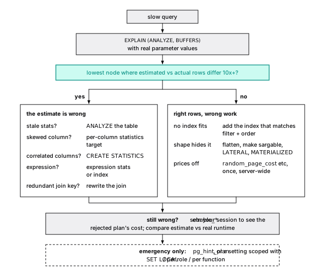
[A method for slow queries](/en/19-explain/#a-method-for-slow-queries) finds the node; [The planner is guessing](/en/20-planner/#basics-chapter-20) has the statistics fixes. If you can reproduce the planner's estimate from `pg_stats`, the statistics are the problem. If you can't even write the formula, because it fell back to a constant, the query shape is. The plan you need is the one from production, with production's parameters, which `auto_explain` logs ([auto_explain logs the plan you can't reproduce later](/en/30-configuration/#auto_explain-logs-the-plan-you-cant-reproduce-later)).
### enable_* shows you the road not taken
Turn an `enable_*` setting off in your session, and `EXPLAIN` shows the plan the planner rejected and what it thought that plan cost. In PostgreSQL 18 a disabled plan type isn't priced with a giant penalty anymore: the planner counts disabled nodes, prefers any plan with fewer, and marks one it had to use anyway. With `enable_seqscan = off` on a table with no other way in:
```text
-> Seq Scan on ev_70k (cost=0.00..2155.00 rows=8780 width=0)
Disabled: true
```
If the rejected plan runs faster but was priced higher, an estimate below it is wrong, or the prices are.
> [!EXAMPLE]- Prove it · lab `20-plans`
>
> ```sql
> set enable_seqscan = off;
> select lab.prove('PostgreSQL 18 marks a forced disabled node instead of adding a huge cost',
> lab.plan_text($$ select count(*) from ev_70k where kind = 'alert' $$) like '%Disabled: true%'
> and est_cost($$ select count(*) from ev_70k where kind = 'alert' $$) < 10000);
> reset enable_seqscan;
> ```
>
> [Full lab script](https://www.flagon.io/books/eight-kilobytes/lab/20-plans.sql)
> [!DANGER] enable_* is a microscope, not a fix
>
> Set `enable_*` only in your own session, to look. A global change silently reshapes every plan on the server, and a setting baked into application code outlives the data that justified it. If you must scope one to a query, use `set local` inside its transaction and write down why.
### pg_hint_plan is for the night a plan flips
Core Postgres has no hints, on purpose ([A hint freezes a plan; fix the estimate instead](/en/20-planner/#a-hint-freezes-a-plan-fix-the-estimate-instead)). The `pg_hint_plan` extension adds them, for the night a production query flips to a bad plan and the statistics fix needs testing first.
Hints live in a `/*+ ... */` comment. They can force scan and join methods or join order, and, most usefully, correct a row estimate (`Rows`), which fixes the cause instead of dictating the plan. Its hint table attaches hints to a query id, so you can fix ORM-generated SQL without touching the app. Every hint is a bet that the data will never change shape: put a ticket next to each one to remove it.
## The short version
- Postgres rewrites your query before costing it. Don't hand-optimize what it already does.
- Join estimates multiply, so errors compound up the tree: a redundant tenant condition made 2,000,000 rows look like 2 and cost 165 times the pages.
- Index scan cost follows correlation squared. On ordered data an index scan won out to 65% of the table, so the 5% rule of thumb is wrong both ways.
- Join search is exhaustive up to 8 explicit `JOIN`s (`join_collapse_limit`) or 11 comma-listed tables, roughly tripling per table; at 12 the genetic optimizer takes over.
- Nested loops win small and lose badly when the outer estimate is low.
- User functions are `PARALLEL UNSAFE` until you mark them. JIT bets on the estimate; turn it off on OLTP primaries.
- When a plan is wrong, check the estimate, then the shape, the index, the prices. `pg_hint_plan` is for emergencies.
## Further reading
- [Planner/Optimizer](https://www.postgresql.org/docs/18/planner-optimizer.html), PostgreSQL documentation. Path generation, the three join strategies, and when GEQO takes over.
- [Parallel Query](https://www.postgresql.org/docs/18/parallel-query.html) and [JIT](https://www.postgresql.org/docs/18/jit.html), PostgreSQL documentation. Parallel safety rules and the JIT cost thresholds, from the source.
- [Access Path Selection in a Relational Database Management System](https://courses.cs.duke.edu/compsci516/cps216/spring03/papers/selinger-etal-1979.pdf), Selinger et al., SIGMOD 1979. The paper behind cost-based access paths and dynamic-programming join search.
- [How Good Are Query Optimizers, Really?](https://www.vldb.org/pvldb/vol9/p204-leis.pdf), Leis et al., PVLDB 2015. Measured on PostgreSQL: cardinality errors, growing with each join, matter far more than the cost model.
- [pg_hint_plan](https://github.com/ossc-db/pg_hint_plan), NTT OSS Center. The hint extension and its hint table.